The Twitter_Suggest Follow Model (The Barabasi-Albert Model)
The twitter_suggest (or preferential_global) follow model is based on the work of Barabasi & Albert with preferential attachment in networks. Preferential attachment occurs when a resource is distributed preferentially to those who already have more. Those who have (x) get more (x). In the twitter_suggest follow model an agent with many followers will get more followers.
Twitter_suggest may be implemented three different ways, each of which is outlined below:
- Classic Barabasi
- Non-Classic Barabasi
- Other (without Barabasi)
Classic Barabasi
The Classic Barabasi configuration is one in which new agents entering the network make exactly one connection with another agent. The new agent will chose to connect to the agent who has the most followers. To model this we set agent follow_rates to zero, so that the only follow decision in the network is made by the entering agent. It should be noted that allowing an agent to follow_back or follow_through_retweets may permit the agent to follow even though their follow_rate is zero.
Constructing The Network
Our starting point is the INFILE.yaml created in Tutorial 3. The INFILE.yaml we create in this example can be found for reference in the hashkat/docs/tutorial_input_files/tutorial04_classic_barabasi.
To run the Classic Barabasi configuration, we set:
- follow_model: twitter_suggest
- use_barabasi: true
- barabasi_connections: 1
- 'Standard' (agent_type) follow_rate: 0
Until now we've had the number of agents within the network remain constant. Now we will have the number of agents increase over time, by setting initial_agents to 10, and max_agents to 1000.
For simplicity, we will only use 'Standard' agent_types. It is imperative we set the 'Standard' agent's follow_rate to 0.0.
analysis:
  initial_agents:
    10
  max_agents:
    1000
  max_time:
    1000
  max_analysis_steps:
    unlimited
  max_real_time:
    1
  enable_interactive_mode:
    false
  enable_lua_hooks: # Defined in same file as interactive_mode. Can slow down simulation considerably.
    false
  lua_script: # Defines behaviour of interactive mode & lua hooks
    INTERACT.lua
  use_barabasi:
    true
  barabasi_connections: # number of connections we want to make when use_barabasi == true
    1
  barabasi_exponent:
    1
  use_random_time_increment:
    true
  use_followback:
    false
  follow_model:
    twitter_suggest

  model_weights: {random: 0.0, twitter_suggest: 0.0, agent: 0.0, preferential_agent: 0.0, hashtag: 0.0}
              # model weights ONLY necessary for follow method 'twitter'
  stage1_unfollow:
    false
  unfollow_tweet_rate:
    10000
  use_hashtag_probability:
    0.5
Note items after # are comments to assist the user and are ignored by the compiler.
In the rates subsection of INFILE.yaml, we will change the 'add' rate to 1.0, meaning one agent will be added to the network per simulated minute.
rates:
  add: {function: constant, value: 1.0}
Now we look at follow_ranks. Generally, agents are grouped into 'bins' for data collection. Many agents are placed in a bin based on their similarity (ie similar number of tweets, retweets & followers).
tweet_ranks:
  thresholds: {bin_spacing: linear, min: 10, max: 500, increment: 10}

retweet_ranks:
  thresholds: {bin_spacing: linear, min: 10, max: 500, increment: 10}

follow_ranks:
# MUST be adjusted for max_agents for simulations which implement the twitter_suggest and/or preferential_agent follow models
  thresholds: {bin_spacing: linear, min: 0, max: 10000, increment: 1}
  weights:    {bin_spacing: linear, min: 1, max: 10001, increment: 1}
The follow_ranks are essential to the twitter_suggest follow model because new following is based on an agent's existing number of followers. Therefore, we must know the exact number of followers an agent has in order to decide if they get new followers. The follow_rank bins change, from 0 to maximum, and to increment by 1. There may still be many agents per bin.
Running and Visualizing The Network
Let's now run this simulation.
After the simulation is run, you may plot the log-log graph of the cumulative-degree_distribution_month_000.dat in Gnuplot by typing these commands:
set style data linespoints
set title 'log of Cumulative-Degree Distribution'
set xlabel 'log(Cumulative-Degree)'
set ylabel 'log(Normalized Cumulative-Degree Probability)'
plot 'cumulative-degree_distribution_month_000.dat' u 3:4 title ''
We should obtain the following graph:

We can see that this produces a fairly linear plot with a negative slope. Agents with few followers are many and agents with many followers are few.
Plotting these data points with a line of best fit up to a log(Cumulative Degree) of 2.5, we can see that this simulation matches a 'scale-free' network, since the line of best fit has a slope between -2 to -3.

The commands to graph this plot in Gnuplot are:
f(x) = m*x + b
set xrange[0:2.5]
set title 'log of Cumulative-Degree Distribution Fit'
set xlabel 'log(Cumulative-Degree)'
set ylabel 'log(Normalized Cumulative Degree Probability)'
fit f(x) 'cumulative-degree_distribution_month_000.dat' u 3:4 every ::1::13 via m,b
plot f(x), 'cumulative-degree_distribution_month_000.dat' u 3:4 title ''
A visualization of this network is shown below:
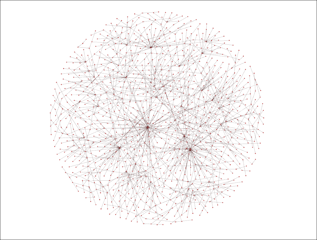
As we can see, we have the highly connected agents at the centre with agents of lower in_degree (i.e. with less followers) on the sides. Classic Barabasi configuration ensures every agent has at least one connection.
Non-Classic Barabasi
The Non-Classic Barabasi configuration is exactly the same as the Classic configuration except that the number of connections new agents make when entering the network is greater than 1.
The configuration file INFILE.yaml used in this example can be found at /hashkat/docs/tutorial_input_files/tutorial04_nonclassic_barabasi.
Constructing The Network
We use the same INFILE.yaml as above except that barabasi_connections is set at 2 instead of 1.
Running and Visualizing The Network
Running the simulation, we produced the visualization shown below:
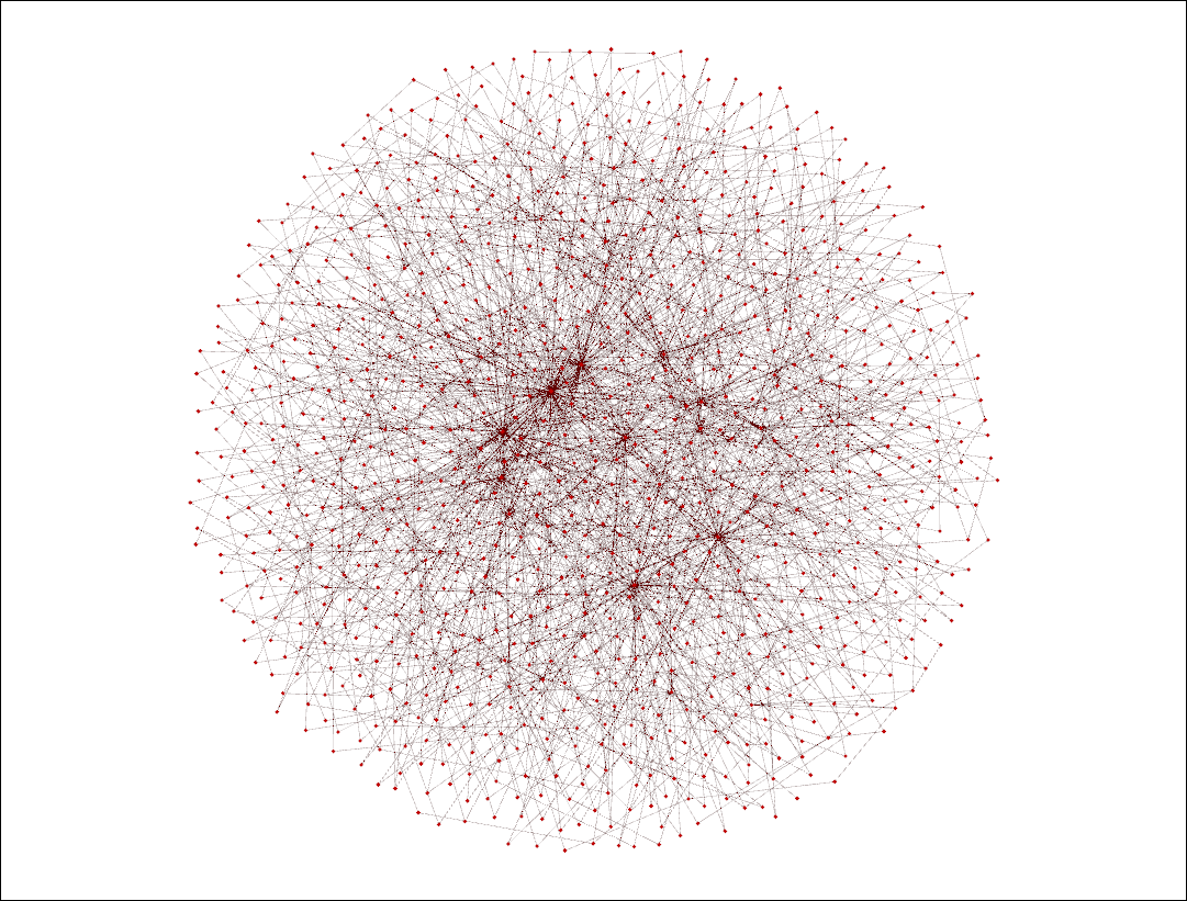
This network similar to the one produced using the Classic Barabasi configuration, with the more connected agents at the centre and those less connected on the sides. However this is a much more connected network since every agent has at least two connections.
Other Twitter_Suggest Models
We shall now run a twitter_suggest follow model network simulation without implementing a Barabasi configuration. The INFILE.yaml used in this example may be found at /hashkat/docs/tutorial_input_files/tutorial04_other.
Constructing The Network
Set:
- use_barabasi: false
- change 'Standard' agent_type follow_rate to 0.01
Running and Visualizing The Network
After running #k@, we produced the following visualization:
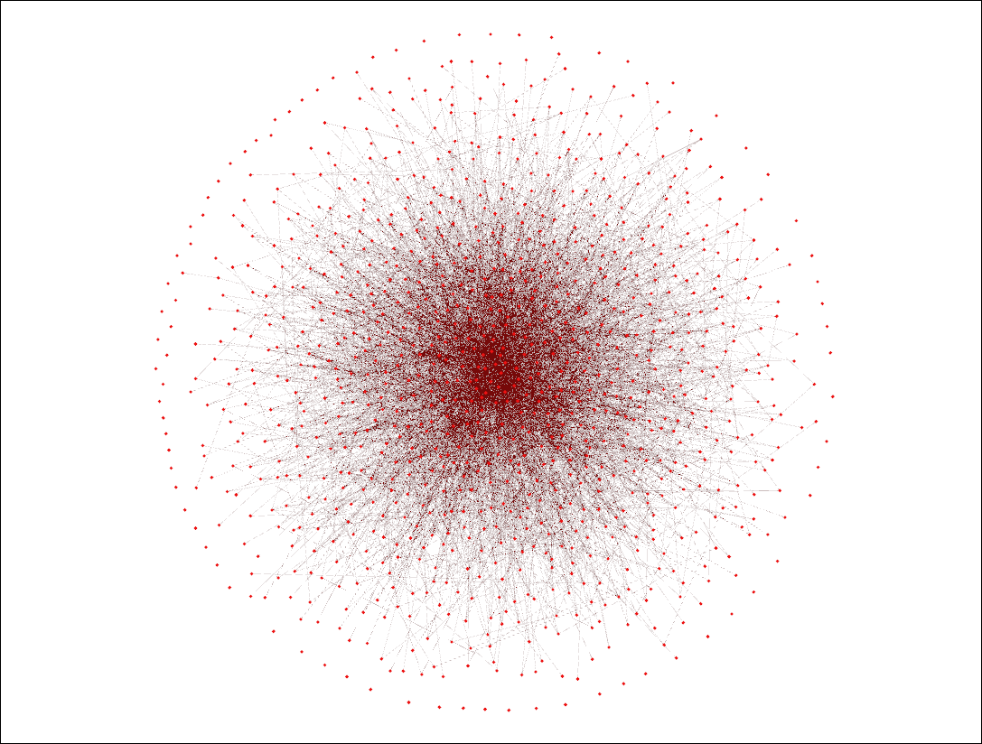
As we can see, we have very highly connected agents in the centre of the visualization and less connected agents on the sides. However, unlike a Barabasi configuration, there is no set number of connections that every new agent must make, which explains the presence of agents with 0 connections at the outside of the circle (on the surface of the sphere).
The output from this simulation is stored in the /hashkat/output/ in the Categories_Distro.dat file.
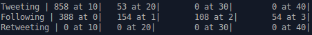
In this file we see that the majority of agents made 10 or fewer tweets. Retweeting was disallowed, so the retweet ranks (bins) have zero agents. We also see how many agents had a certain number of followers. Looking further through this file, we can see that the most followed agent had 86 followers. We verify this by observing the bins above 86 are empty.

A plot of the follow_ranks up to a follow_rank of 15 is shown below:

Next Steps
We have now worked with a few configurations of the twitter_suggest preferential attachment follow model. We encourage you to do your own experiments. In the next tutorial we demonstrate the agent follow_model.