Getting Started
An introduction to #k@, this tutorial will take approximately 20 minutes to complete.
What is a Social Network?
A network as seen through graph theory is a set of users or agents (nodes) and connections between them (edges).
In the real world, a social network is a set of connections made by agents acting voluntarily, for recreational purposes. Unlike, for example, a network set up to connect government offices, or all outlets of General Motors (tm), which can be considered top-down designed networks, (also with proprietary content), social networks are created bottom up, by agents who are NOT obligated to participate or produce signals. Social networks are fluid and unique to the agent.
Within the social network, connected agents receive signals (content) from each other, either in one direction only (Twitter) or bidirectionally (Facebook). For purpose of these tutorials, language appropriate to Twitter will be used.
The goal of #k@ is to simulate the growth of social networks and the propagation of signals within them.
What is #k@?
In the #k@ simulation, the network is set up with a certain number of initial agents and with an add_rate of new agents to the network. The network also has a decay_rate for signals, or time beyond which signals will no longer be retransmitted.
The agents are set up to be of different types, with different preferences. The agents are configured for:
-
The type of agent (standard, celebrity, organization or bot).
-
The agent's characterstics in terms of region, language, and ideology.
-
The type of signal the agent is likely to generate (tweet). Signal types are general, political, humorous, musical. The type of signal affects its scope of retransmission.
-
The type of signal the agent is likely to retransmit.
-
The events that will cause the agent to follow another agent (follow-model and edge creation).
-
The events that will cause the agent to unfollow another agent (edge deletion).
-
Rates (probabilities) are set for each type of behavior. For example, Agent_type A may 50% likely to generate a political tweet and 50% likely to generate a musical tweet. Agent A may tweet once a day, Agent B may tweet 10 times a day.
A simulated time and real time are set for the simulation to run.
The simulation commences.
At each increment in time agents chose: whom to follow; whether or not to generate a signal; the content of the signal; whether or not to retransmit a signal received; and whether or not to unfollow another agent.
At the end of the allotted time, the simulation ceases. Output files are generated and stored in ~/hashkat/output/. The output files may be visualized through third party programs such as Gnuplot, Gephi or Networkx.
What is the Kinetic Monte Carlo (KMC) Method?
Hashkat takes one action per time increment. As the network gets larger, the time increment gets smaller, i.e., if a network with one agent takes an action every hour, a network with 60 agents will take an action every minute, and a network with 3600 agents will take an action every second. This example shows time compression which is dependent on the number of agents.
The Kinetic Monte Carlo (KMC) algorithm compresses the time increment based on the cumulative rate function R (the sum of the rates within the system). The algorithm as used by #k@ is discussed in more detail here.
For #k@, the cumulative rate function R is the sum of the network 'add' rate, and the different agents' 'tweet','follow', and 'retweet' rates. Note: the 'tweet', 'follow', and 'retweet' rates are multiplied by the number of agents of that type in the network.
R = add_rate + T1(tweet_rate1 + follow_rate1 + retweet_rate1)+...+Tn(tweet_raten + follow_raten + retweet_raten)
The default build of #k@ permits 200 different agent_types (n = 200). However, you may wish modify the proportion of each agent_type, i.e. to have 1000 agents of Type_1 (T1 = 1000), but only 10 of Type_2, for a 100:1 ratio Type_1:Type_2.
As time increments, a random number r1 is generated. which will determine which action, of all actions available at that point in time, is taken in the system. A new agent may be added, a tweet made, a retweet made, or an agent may be followed, etc.
The R will change, reflecting new rates in the system (i.e. each new agent enters the systems with a set of their own rates), and time will increment.
If 'use_random_time_increment' in 'INFILE.yaml' is enabled, another random number rt is generated, and time will move forward by:
If it is not enabled, time will move forward by:
The cycle will repeat with a new random number r2 generated.
How to Run #k@
#k@ is written in C++, a compiled (built) language. First one builds the #k@ program.
./build.sh
The build defines the number of Regions, Ideologies, Agent-types, and Preferences the agents may have in the simulated network. For now, we will use the default build, and simply demonstrate how to modify configuration.
After the build one configures the network in INFILE.yaml to give Agents their particular Region, Language, tweet Preferences, follow rates etc.
~/hashkat/INFILE.yaml
When configuration is complete, one runs the simulation:
./run.sh
The simulation generates several output files and a new output directory. Some of the output files are in /hashkat/ and some are in /hashkat/output/.
To run a second simulation in #k@ we need to remove the output files from the first simulation. This process is shown in Tutorial02.
How to Run #k@ For Tutorials
The files we are using in the tutorials are stored separately. To do the simulations shown in the tutorials, for example tutorial01, open:
~/hashkat/docs/tutorial_input_files/tutorial01
you will see 'tutorial01' contains its own file called 'INFILE.yaml', which is the configuration shown in this tutorial. To run the tutorial01 configuration, from inside the directory tutorial_input_files enter:
'~/hashkat/run.sh`
This will not affect the main configuration file of hashkat.
Running a Simple Network
For this first tutorial, we're going to run a simple network. We will add configuration parameters as we progress through the tutorials to obtain a robust and complex simulation. More information about the input parameters is available on the Input page.
In this tutorial, we will have a constant (unchanging) number of agents (add_rate = 0), 1000 initial agents (n = 1000), and one agent_type with a 'tweet' rate of 0.0001 per minute. The simulation will run for 100,000 simulated minutes or 1 minute real time. The 'follow', 'retweet', and 'unfollow' rates are set to zero. Therefore:
R = 0 + (1000)(0.0001 + 0 + 0) = 0.1
Run the simulation by typing in the command:
../run.sh
You may refer to Installation for more information on running a simulation for the first time and using the command line.
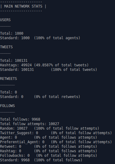
When running this program, you will see something similar to this on the screen which shows data at particular points in the simulation:
| Simulation Time (min) | Users | Follows | Tweets | Retweets | Unfollows | R | Real Time (s) |
|---|---|---|---|---|---|---|---|
| 9.93e+04 | 1.00e+03 | 1.00e+04 | 0.00e+00 | 0.00e+00(0.00e+00) | 0.00e+00 | 1.00e-01 | 2.25e+00 |
Note we can see both 'Retweets' and a number beside it in brackets. This is the number of 'active' tweets, which are signals that have not yet 'decayed' and are eligible to be retransmitted.
We see that at simulated time of 99,300 minutes, there were still 1,000 agents in the network (0 = add_rate), with 10,000 follows, 0 tweets, 0 retweets, and 0 unfollows. The cumulative rate function was 0.1, and the real time that elapsed was 2.25 seconds.
Once the simulation is concluded, output files will be created and the real time elapsed will be displayed on the screen in milliseconds.
Output of a Simple Network
The simulation creates several output files, one in the hashkat directory and most in a new output directory. The new files include:
~/hashkat/network_state.dat~/hashkat/output/DATA_vs_TIME
The configuration file INFILE.yaml is also automatically copied into the output directory for future reference.
To go into the output directory and view its contents use the commands
cd output
ls
This lists all the files of information collected from the simulation. Let's look at some of this data. Go into the main_stats.dat file by typing in the command
nano main_stats.dat
Nano will display the contents of main_stats.dat as text. We can see the 'in-degree distribution' (an agent's followers), 'out-degree distribution' (those an agent follows), and 'cumulative-degree distribution' (both an agent's followers & following) for ALL the agents, by simulated month.
The agents in this simulation had a follow rate set at 0.0001 per simulated minute. In 100,000 simulated minutes we would expect each agent to follow approximately 10 agents, and be followed by the same number. Therefore, we can expect most agents to have an in-degree value of 10, an out-degree value of 10, and a cumulative-degree value of 20.
To plot the results, we may use gnuplot. To access gnuplot, type in the command:
gnuplot
The most up-to-date data is in 'month002'. To plot the in-degree, out-degree, and cumulative-degree distributions for this month on the same graph with appropriate axis labels and a title, type in the following:
set style fill transparent solid 0.5 noborder
set title 'Agent Degree Distributions'
set xlabel 'Degree'
set ylabel 'Normalized Degree Probability'
plot 'in-degree_distribution_month_002.dat' u 1:2 lc rgb 'red' with filledcurves title 'In-Degree',
'out-degree_distribution_month_002.dat' u 1:2 lc rgb 'goldenrod' with filledcurves title 'Out-Degree',
'cumulative-degree_distribution_month_002.dat' u 1:2 lc rgb 'blue' with filledcurves
title 'Cumulative-Degree'
Giving us:

As expected, most agents have an in-degree of about 10, an out-degree of about 10, and a cumulative degree of about 20.
Note that you can save your plots by typing in the command:
set output <filename>
when you first start up Gnuplot and prior to actually plotting the data.
Visualizing a Simple Network
You may also use the data you collected to visualize your simulated network. We will discuss how to do so using Gephi here. A more in-depth discussion can be found on the Visualization page.
Entering Gephi, open the graph file network.gexf found in the 'output' directory of your simulation. Press 'OK' for the 'Import report' window that pops up, and you will now see a rough outline of your network. Under the 'Partition' subheading on the left side of the page, press the 'refresh' symbol, and choose the partition parameter 'Label' and click 'Apply'. You are now free to choose a layout for this network directly below the 'Apply' button you just pushed, and can run it for a few seconds. The following visualization was made using the 'Fruchterman Reingold' and 'Clockwise Rotate' layout:
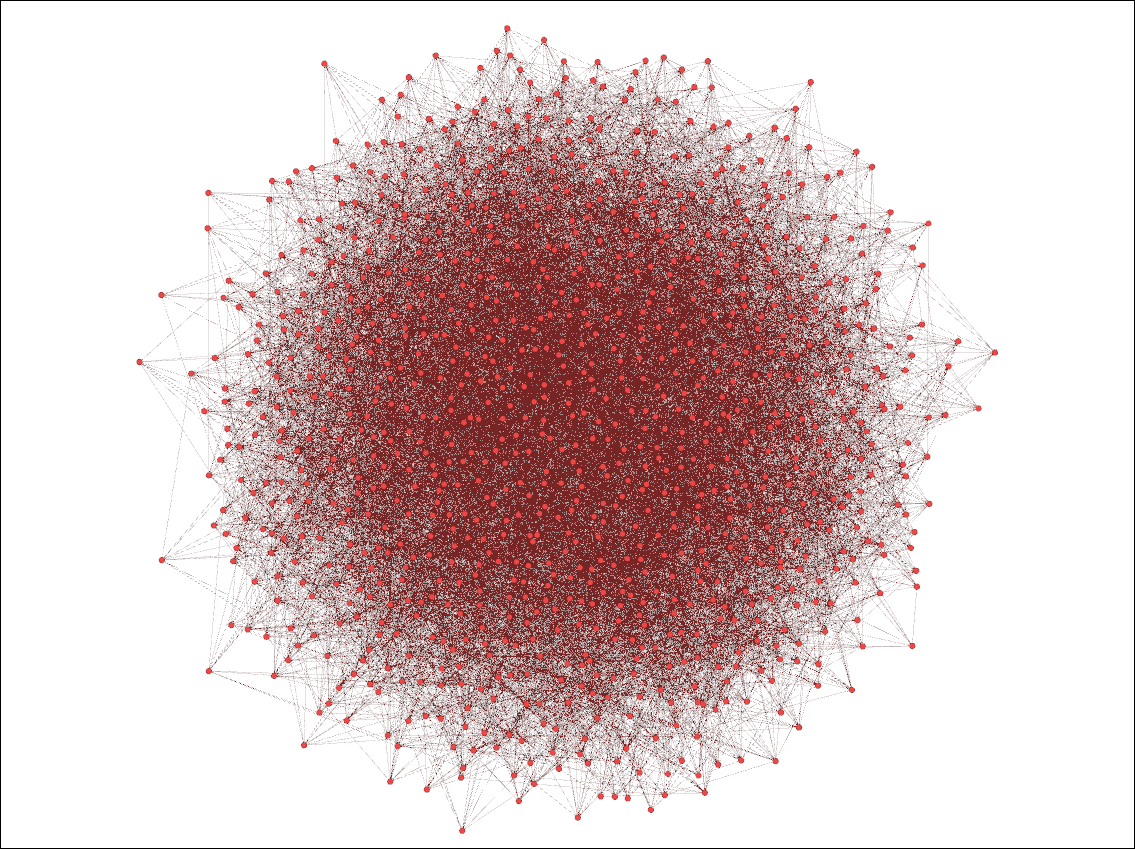
We can see that these agents (the red nodes) are randomly connected within this network simulation we created, with the highly connected agents at the centre of the visualization and the agents with less connections on the sides.
Next Steps
You have now completed your first tutorial using #k@, where you ran a simple network simulation, studied its output, and visualized it.
The input file used for this tutorial can be found in the hashkat directory in the docs/tutorial_input_files directory under tutorial01 as well as here, so the main configuration file, ~/hashkat/INFILE.yaml has not yet been changed.
Feel free to move on to the next tutorial, where we will discuss restarting a network.